
Noise, vibration and earthquakes: a primer built around Taipei 101
Published:
These are condensed lecture notes from my session on earthquakes for a course on noise and vibration in environmental engineering. The thread running through them is one building: Taipei 101, which stands in one of the most seismically active and typhoon-exposed places on Earth.
The building
- Foundation: 380 piles driven about 80 m down through the soft clay of the Taipei Basin into bedrock.
- Core: a steel-reinforced concrete core carries the vertical load.
- Tuned mass damper (TMD): a 660-tonne steel sphere hung between the 87th and 92nd floors, tuned to the tower’s natural frequency (about 0.14 Hz, a period of roughly 7 s). When the tower sways one way, the sphere lags and swings the other way, and hydraulic dampers turn that motion into heat. Reductions in sway of up to about 40% are commonly quoted.
1. Measuring the threat: magnitude and energy
Earthquakes follow elastic rebound (Reid, 1906): a locked fault stores strain as the plates keep moving, the rock breaks when stress exceeds the fault’s frictional strength, and the stored energy leaves as seismic waves.
The size of the event is the seismic moment
\[M_0 = \mu A D\]where \(\mu\) is the shear modulus (about \(3 \times 10^{10}\) N/m² for crustal rock), \(A\) the rupture area and \(D\) the average slip. Moment magnitude is
\[M_w = \tfrac{2}{3}\log_{10} M_0 - 6.07 \quad (M_0 \text{ in N·m}).\]Worked example: 2004 Sumatra–Andaman. With \(L = 1{,}300\) km, \(W = 150\) km, \(D = 10\) m and \(\mu = 3.5 \times 10^{10}\) N/m²:
- \(A = 1.95 \times 10^{11}\) m²
- \(M_0 = 6.8 \times 10^{22}\) N·m
- \[M_w = \tfrac{2}{3}(22.83) - 6.07 \approx 9.15\]
- Radiated energy, \(\log_{10} E = 4.8 + 1.5 M_w\), gives \(E \approx 3.4 \times 10^{18}\) J.
Worked example: slip for an M7.1. The 31 March 2002 offshore earthquake shook Taipei hard enough that two construction cranes fell from Taipei 101, killing five people, even though the epicentre was far away. For an \(M_w\) 7.1 on a 30 × 20 km fault: \(M_0 = 10^{1.5(7.1 + 6.07)} \approx 5.7 \times 10^{19}\) N·m, so \(D = M_0 / (\mu A) \approx 3.2\) m.
2. The signal: waves and frequency
| Wave | Type | Particle motion | Damage potential |
|---|---|---|---|
| P | Body | Push–pull, along the travel direction | Low, the first jolt |
| S | Body | Shear, across the travel direction; no travel through liquids | Moderate |
| Love | Surface | Horizontal side-to-side | High |
| Rayleigh | Surface | Elliptical rolling | High |
\(V_P > V_S >\) surface waves, so the P wave always arrives first. That gap is what earthquake early-warning systems exploit.
Site class. Building codes classify ground by \(V_{S30}\), the time-averaged shear-wave velocity of the top 30 m. Simplified classes (ASCE 7-16 style; ASCE 7-22 adds intermediate classes such as BC, CD and DE):
| Class | Ground | \(V_{S30}\) (m/s) |
|---|---|---|
| A | Hard rock | > 1,500 |
| B | Rock | 760–1,500 |
| C | Very dense soil / soft rock | 370–760 |
| D | Stiff soil | 180–370 |
| E | Soft clay | < 180 |
| F | Liquefiable, organic, etc. | site-specific analysis |
Much of the Taipei Basin is soft soil that amplifies shaking, which is why a distant earthquake can still be dangerous there.
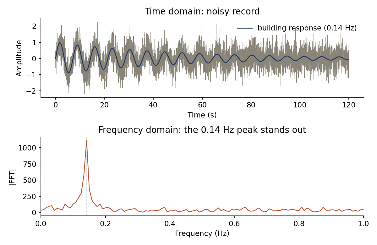
Resonance. A rough rule gives a building period of \(T \approx 0.1N\) seconds for \(N\) storeys. If the ground shakes near the building’s own frequency, each cycle adds to the sway. The figure above shows the standard way to find that frequency in a noisy record: a Fourier transform.
import numpy as np

fs, f_building = 50.0, 0.14                 # sampling rate (Hz), building frequency (Hz)
t = np.arange(0, 120, 1 / fs)
signal = np.sin(2 * np.pi * f_building * t) * np.exp(-0.02 * t)
record = signal + 0.5 * np.random.normal(size=t.size)   # add "cultural" noise

f = np.fft.rfftfreq(t.size, 1 / fs)
amp = np.abs(np.fft.rfft(record))
print(f"Peak at {f[np.argmax(amp[1:]) + 1]:.3f} Hz")
3. Site risk: deterministic hazard and design spectra
A deterministic seismic hazard analysis (DSHA) has four steps:
- Identify the seismic sources (active faults within roughly 100–200 km).
- Choose the largest credible earthquake on each, usually from fault length.
- Use a ground-motion prediction equation (GMPE) to estimate shaking at the site from magnitude and distance.
- Take the worst case as the design basis.
Codes then turn hazard into a design response spectrum, the peak acceleration felt by buildings of different natural periods:
- \(T < T_0\): \(S_a = S_{DS}(0.4 + 0.6\,T/T_0)\)
- \(T_0 \le T \le T_S\): \(S_a = S_{DS}\)
- \(T > T_S\): \(S_a = S_{D1}/T\), with \(T_S = S_{D1}/S_{DS}\) and \(T_0 = 0.2\,T_S\)
Tall, flexible buildings sit on the \(1/T\) branch: they feel lower acceleration but larger displacement.
Liquefaction. Saturated loose sand can lose its strength when shaken. The demand is the cyclic stress ratio
\[CSR = 0.65 \left(\frac{a_{max}}{g}\right)\left(\frac{\sigma_{vo}}{\sigma'_{vo}}\right) r_d,\]and liquefaction is expected where \(FS = CRR/CSR \le 1\). Deep piles to bedrock, as at Taipei 101, avoid relying on the weak upper layers at all.
4. Mitigation
A building’s motion follows \(m\ddot{x} + c\dot{x} + kx = F(t)\). Engineers either move the natural frequency away from the shaking (change \(k\) or \(m\)) or add damping (\(c\)).
- Tuned mass damper: absorbs energy inside a tall, flexible structure, and helps with wind as well as earthquakes. A pendulum suits a very low frequency because \(f = \frac{1}{2\pi}\sqrt{g/L}\) depends only on cable length.
- Base isolation: decouples a short, stiff building from the ground.
- Code factors: the response modification factor \(R\) allows controlled ductile damage, and the importance factor \(I_e\) (1.25–1.5) raises design forces for hospitals and other essential facilities.
- Beyond the building: early warning (seconds to tens of seconds) and land-use rules that keep tall buildings off the softest ground and away from active fault traces.
import numpy as np

def response(t, zeta, fn):
    wn = 2 * np.pi * fn
    return np.exp(-zeta * wn * t) * np.cos(wn * t)   # free vibration of a damped oscillator

t = np.linspace(0, 60, 2000)
low = response(t, 0.02, 0.14)    # ordinary building, 2% damping
high = response(t, 0.15, 0.14)   # with added damping, 15%
Common questions
Why 30 m for \(V_{S30}\)? It is a convention: the stiffness of the top 30 m is the main control on amplification and is affordable to measure. Deeper layers still matter for long-period buildings.
Is there a shortcut for design spectra? In practice engineers look up \(S_{DS}\) and \(S_{D1}\) from national hazard maps for the site’s coordinates. In class you should still know which spectrum branch applies for a given period.
What if the building frequency matches the ground? Shift it: add stiffness (bracing, shear walls) to raise the frequency, or, less commonly, add mass to lower it, or add damping.