
Active faults and the b-value: a classroom exercise
Published:
A short exercise I use in geohazards classes: how we recognise active faults, and how the Gutenberg–Richter b-value turns an earthquake catalogue into a recurrence model for hazard analysis.
What counts as an active fault?
A fault is usually called active if it has moved in the Holocene (the last 11,700 years) or, for some agencies, the Late Pleistocene. Evidence comes from mapped surface ruptures, trenches across the fault, dated sediments, geomorphology and geophysical images of the subsurface.
Thailand’s Department of Mineral Resources recognises 16 active fault zones: Mae Chan, Mae Hong Son, Mae Tha, Thoen, Phayao, Mae Ing, Mae Lao, Wiang Haeng, Pua, Uttaradit, Moei, Three Pagodas, Sri Sawat, Ranong, Khlong Marui and Phetchabun. Several of them, including the Phayao zone that produced the 5 May 2014 Mae Lao (Chiang Rai) earthquake (Mw 6.5 from our regional moment tensor; Noisagool et al., 2016), are the subject of our own geophysical work.
The Gutenberg–Richter relation
\[\log_{10} N = a - bM\]- \(N\) is the number of earthquakes with magnitude \(\ge M\) in a region and time period.
- \(a\) measures the overall rate of seismicity.
- \(b\) describes how many small earthquakes there are for each large one. It is usually close to 1.0 but varies with stress and crustal heterogeneity.
Exercise: fit the b-value
Copy the sample catalogue into a spreadsheet:
| Magnitude M | Events in bin | Cumulative N (≥ M) | log₁₀ N |
|---|---|---|---|
| 3.0 | 500 | 832 | 2.92 |
| 3.5 | 200 | 332 | 2.52 |
| 4.0 | 80 | 132 | 2.12 |
| 4.5 | 35 | 52 | 1.72 |
| 5.0 | 12 | 17 | 1.23 |
| 5.5 | 4 | 5 | 0.70 |
| 6.0 | 1 | 1 | 0.00 |
- Build the cumulative column by summing from the largest magnitude upwards.
- Take log₁₀ of the cumulative counts.
- Plot log₁₀ N against M and add a linear trendline with its equation.
- The slope is −b and the intercept is a.
- Report a and b and compare b with the global average of about 1.0.
For this catalogue a least-squares fit gives a ≈ 5.87 and b ≈ 0.95.
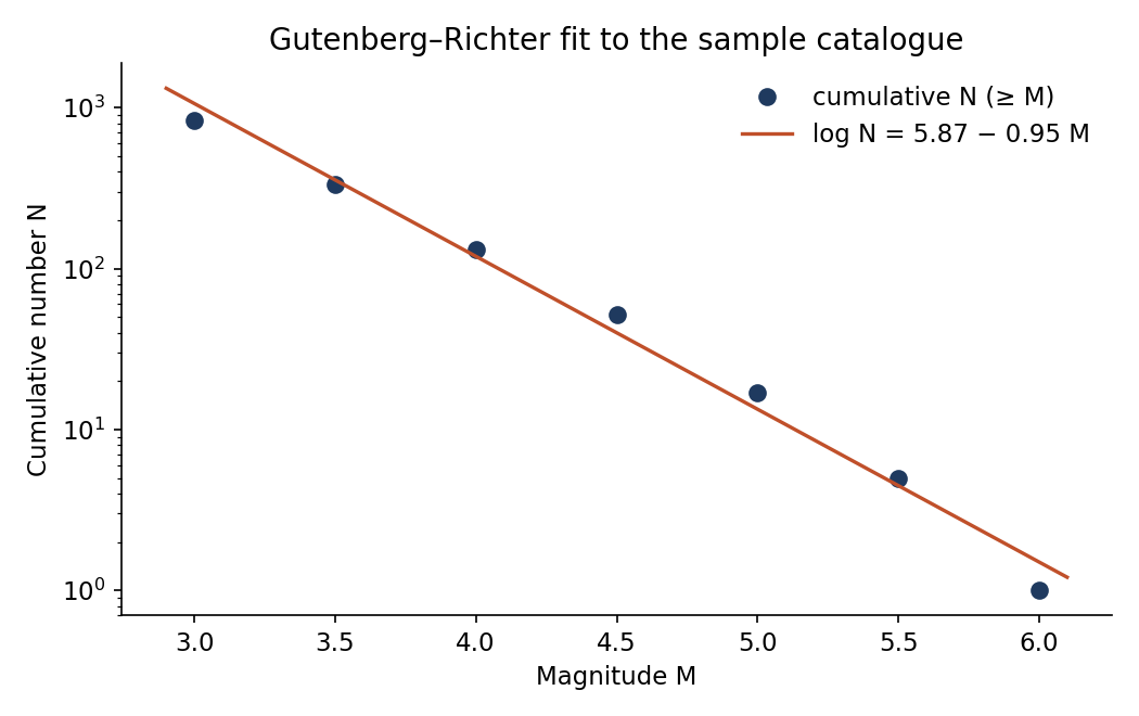
The same fit in Python:
import numpy as np

M = np.array([3.0, 3.5, 4.0, 4.5, 5.0, 5.5, 6.0])
N = np.array([832, 332, 132, 52, 17, 5, 1])
slope, a = np.polyfit(M, np.log10(N), 1)
print(f"a = {a:.2f}, b = {-slope:.2f}")
Least squares is the classroom method. For research, use the maximum-likelihood estimate (Aki, 1965) above the catalogue’s magnitude of completeness, because a straight-line fit gives too much weight to the few large events.
Going further: clustering epicentres
Machine-learning methods such as k-means can group epicentres into clusters that sometimes follow fault segments. It is a useful exploratory tool, but clusters are not faults: always check them against geology and focal mechanisms.
import numpy as np
from sklearn.cluster import KMeans

rng = np.random.default_rng(42)
segment_a = rng.normal(size=(50, 2)) * 0.2 + [99.9, 19.7]
segment_b = rng.normal(size=(50, 2)) * 0.15 + [100.3, 20.2]
epicentres = np.vstack([segment_a, segment_b])     # (longitude, latitude)

km = KMeans(n_clusters=2, random_state=0, n_init="auto").fit(epicentres)
print(km.cluster_centers_)